【2023年】第30天 Supervised Learning with TensorFlow 2（用TensorFlow进行监督学习 2）

1.Basic regression: Predict fuel efficiency

基本回归： 预测燃油效率 （这是tensorflow官网的一个例子，我们进一步剖析）

In a regression problem, the aim is to predict the output of a continuous value, like a price or a probability.
在回归问题中，目的是预测一个连续值的输出，如价格或概率。
Contrast this with a classification problem, where the aim is to select a class from a list of classes (for example, where a picture contains an apple or an orange, recognizing which fruit is in the picture).
这与分类问题形成鲜明对比，后者的目的是从一个类别列表中选择一个类别（例如，一张图片包含一个苹果或一个橙子，识别图片中的哪个水果）。
This tutorial uses the classic Auto MPG(miles per gallon) dataset and demonstrates how to build models to predict the fuel efficiency of the late-1970s and early 1980s automobiles.
本教程使用经典的汽车MPG数据集，演示了如何建立模型来预测1970年代末和1980年代初的汽车的燃油效率。
https://archive.ics.uci.edu/dataset/9/auto+mpg 数据集地址
MPG(miles per gallon) 油耗(英里每加仑)
To do this, you will provide the models with a description of many automobiles from that time period.
要做到这一点，你将为这些模型提供该时期的许多汽车的描述。
This description includes attributes like cylinders, displacement, horsepower, and weight.
这种描述包括气缸、排量、马力和重量等属性。

import matplotlib.pyplot as plt
import numpy as np
import pandas as pd
import seaborn as sns

np.set_printoptions(precision=3, suppress=True)
# 这行代码设置了在打印数组时的格式选项。
# precision 参数指定了小数精度，即小数点后保留的位数；
# suppress 参数指定是否要使用科学计数法。
# 这里的设置将会使所有的浮点数只会输出三位小数，并且不使用科学计数法。

import tensorflow as tf

from tensorflow import keras
from tensorflow.keras import layers

print(tf.__version__)

# Get the data
# First download and import the dataset using pandas:
url = 'http://archive.ics.uci.edu/ml/machine-learning-databases/auto-mpg/auto-mpg.data'
# 定义一个字符串变量 url，保存数据集的下载链接。
column_names = ['MPG', 'Cylinders', 'Displacement', 'Horsepower', 'Weight', 'Acceleration', 'Model Year', 'Origin']
# 定义一个列表 column_names，其中包含了我们将要读取的数据集的每一列的名称，共8列。
raw_dataset = pd.read_csv(url, names=column_names,
                          na_values='?', comment='\t',
                          sep=' ', skipinitialspace=True)
# Pandas 的 read_csv() 函数用于读取 CSV 格式的文件并将其转换为 DataFrame 对象。在此例中，我们传递了以下参数：
# url: 数据集的下载链接。
# names: 包含每一列名称的列表。
# na_values: 指定缺失值的标识符，这里用问号 ? 表示。
# comment: 指定注释的标识符，这里用制表符 \t 表示。
# sep: 指定列之间的分隔符，这里用空格 ' ' 表示。
# skipinitialspace: 指定是否跳过列与分隔符之间的初始空格，默认为 False。
# 最终，该函数将返回一个 DataFrame 对象 raw_dataset，包含了数据集的所有行和列。

# raw_dataset.copy() 复制数据集 raw_dataset，返回一个新的数据集副本。
dataset = raw_dataset.copy()
# 使用 .tail() 方法显示数据集最后几行，默认是5行。该方法可以快速观察数据集的结尾部分，以便检查数据是否完整或有缺失值。
dataset.tail()

运行结果：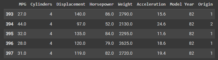

# Clean the data
# The dataset contains a few unknown values:
# 检查数据集中的哪些元素是缺失的，然后计算每一列的缺失值的数量。
dataset.isna().sum()

The dataset contains a few unknown values:
该数据集包含一些未知值：
运行结果：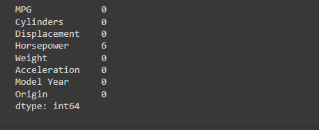

dataset = dataset.dropna()

The “Origin” column is categorical, not numeric.
“Origin” 列实际上代表分类，而不仅仅是一个数字。所以把它转换为独热码 （one-hot）

# dataset['Origin'] 表示选取数据集 dataset 中名为 Origin 的列，map() 方法对该列进行操作。
dataset['Origin'] = dataset['Origin'].map({1: 'USA', 2: 'Europe', 3: 'Japan'})
# {1: 'USA', 2: 'Europe', 3: 'Japan'} 是一个字典，表示原始数据集中 Origin 列中的数值类型及其对应的字符串类型。其中，数字 1 对应字符串 'USA'，数字 2 对应字符串 'Europe'，数字 3 对应字符串 'Japan'。
# 将 map() 方法得到的结果重新赋值给 dataset['Origin']，即将原始数据集中 Origin 列中的数值类型映射成对应的字符串类型。

# 这段程序的作用是将数据集中的 Origin 列中的字符串类型转化为数值类型。
# pd.get_dummies(dataset, columns=['Origin'], prefix='', prefix_sep='') 表示使用 Pandas 库中的 get_dummies() 函数对数据集 dataset 中名为 Origin 的列进行操作，生成新的虚拟变量（dummy variable）。prefix='' 和 prefix_sep='' 参数表示不为生成的虚拟变量设置前缀和前缀分隔符。
dataset = pd.get_dummies(dataset, columns=['Origin'], prefix='', prefix_sep='')
dataset.tail()
# 在转化后，生成的虚拟变量列名与原始字符串类型相同，每个虚拟变量列都是二进制的，如果某一行数据的 Origin 值为该列对应的字符串类型，则该列对应的二进制数为 1，否则为 0。例如，若某行数据的 Origin 值为 'USA'，则生成的虚拟变量列名为 'USA'，该列所有非零数据均为 1。

运行结果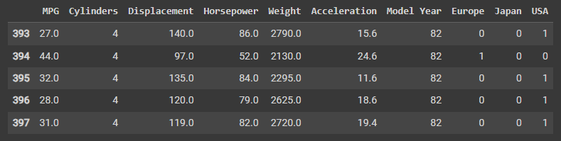

# Split the data into training and test sets
# Now, split the dataset into a training set and a test set. You will use the test set in the final evaluation of your models.
train_dataset = dataset.sample(frac=0.8, random_state=0)
# 该行代码使用 pandas 库中的 sample() 方法，从原始数据集 dataset 中随机抽取 80% 的样本构成训练数据集，并将其存储在 train_dataset 变量中。其中，frac=0.8 表示要抽取的比例为 80%，random_state=0 则是随机数生成器的种子，确保每次运行程序时得到的结果都相同。
test_dataset = dataset.drop(train_dataset.index)
# 该行代码使用 pandas 库中的 drop() 方法，删除训练数据集 train_dataset 中的索引对应的样本，并将剩余的样本构成测试数据集，并将其存储在 test_dataset 变量中。
# 具体来说，train_dataset.index 返回训练数据集中的所有索引值，dataset.drop() 方法会删除这些索引值对应的行，即剩余的行就是测试数据集的数据。

# Inspect the data 检查数据
# Review the joint distribution of a few pairs of columns from the training set.
# 快速查看训练集中几对列的联合分布。
# The top row suggests that the fuel efficiency (MPG) is a function of all the other parameters. 
# 最上面一行表明，燃油效率（MPG）是所有其他参数的一个函数。
#  The other rows indicate they are functions of each other.
# 其他行表示它们是彼此的函数。
sns.pairplot(train_dataset[['MPG', 'Cylinders', 'Displacement', 'Weight']], diag_kind='kde')
# 选择'train_dataset'数据集中的'MPG', 'Cylinders', 'Displacement', 'Weight'四个变量
# 对角线上绘制核密度估计图，也可以设置为'histrogram'绘制直方图

运行结果：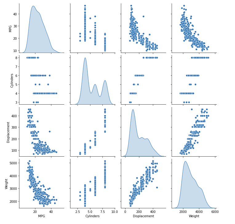

核密度估计图（Kernel Density Estimation, KDE）是一种用于可视化连续变量分布的图形工具。它可以帮助我们理解数据的分布，并在直方图等图形不能清晰表示数据分布时发挥重要作用。

KDE通过将每个数据点周围的“内核”（kernel）组合起来来估计概率密度函数，从而创建平滑的曲线，以显示观察数据的相对频率。

KDE图的x轴表示变量值，y轴表示概率密度。曲线下面积总和为1，因此可以看做是连续变量的概率密度函数估计。核密度估计图通常与直方图一起使用，以提供更全面的数据分布信息。

Let’s also check the overall statistics. Note how each feature covers a very different range:
我们也来检查一下整体的统计数据。请注意每个特征所涵盖的范围是非常不同的：

# describe(): 对数据集进行描述性统计分析，计算如下指标：样本数量（count）、均值（mean）、标准差（std）、最小值（min）、25%分位数（25%）、50%分位数（50%）、75%分位数（75%）和最大值（max）
# transpose(): 将计算出来的统计信息行列转换，以得到更直观的表现形式
train_dataset.describe().transpose()
# 因此，该行代码执行后会输出一个表格，其中每一行代表一个数值型变量，每一列显示一个统计指标的值。
# 例如，第一行的count表示'MPG'变量在数据集中的非缺失值数量，mean表示'MPG'变量的平均值，std表示标准差，min和max则分别表示'MPG'变量在数据集中的最小值和最大值。

运行结果：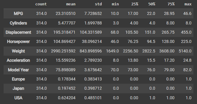

# Split features from labels
# Separate the target value—the "label"—from the features. 
# This label is the value that you will train the model to predict.
# 复制训练集和测试集数据，以便对它们进行修改，同时保留原始数据集。
train_features = train_dataset.copy()
test_features = test_dataset.copy()

# 从复制后的训练集和测试集中删除 MPG 列，并将其保存到 train_labels 和 test_labels 变量中。
train_labels = train_features.pop('MPG')
test_labels = test_features.pop('MPG')

这里使用了 DataFrame 的 pop 方法，它可以删除指定的列并返回该列的值，因此 train_labels 和 test_labels 变量分别保存了训练集和测试集中的 MPG 列。

# Normalization 归一化
# In the table of statistics it's easy to see how different the ranges of each feature are:
train_dataset.describe().transpose()[['mean', 'std']]
# 调用 train_dataset 的 describe 方法，它会对数据集中所有数值型特征列进行统计描述，包括计数、均值、标准差、最小值、最大值和四分位数等。
# 使用 transpose 方法将统计描述结果进行转置，使每个特征列的描述信息成为一行，方便查看。
# 从转置后的结果中选择均值和标准差两列，即 ['mean', 'std']，并以这两列为列索引显示结果，这样可以更加清晰地查看均值和标准差的值。

运行结果：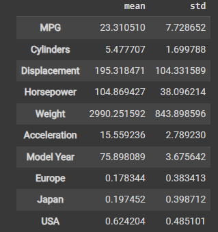

It is good practice to normalize features that use different scales and ranges.
对使用不同尺度和范围的特征进行标准化是一个好的做法。
One reason this is important is because the features are multiplied by the model weights.
这很重要的一个原因是，特征要乘以模型的权重。
So, the scale of the outputs and the scale of the gradients are affected by the scale of the inputs.
所以，输出的规模和梯度的规模都受到输入规模的影响。
Although a model might converge without feature normalization, normalization makes training much more stable.
虽然一个模型在没有特征归一化的情况下可能会收敛，但归一化使训练更加稳定。

# The Normalization layer
# The tf.keras.layers.Normalization is a clean and simple way to add feature normalization into your model.
# The first step is to create the layer:
normalizer = tf.keras.layers.Normalization(axis=-1)

这段代码创建了一个 Keras 层（Layer）：
（1）创建了一个 Normalization 类的对象 normalizer，用于对输入数据进行归一化处理。
（2）axis=-1 参数指定了进行归一化处理的轴，这里为最后一个维度，即对每个样本中的每个特征进行归一化处理。
（3）在模型训练过程中，该层将会自动计算特征的均值和标准差，并用这些值对输入数据进行归一化处理。

归一化处理是一种常见的数据预处理技术，它可以将数据缩放到一个固定的范围内，以便更好地进行训练和预测。在深度学习中，归一化处理可以帮助加速模型的收敛速度，提高模型的泛化能力。

# Then, fit the state of the preprocessing layer to the data by calling Normalization.adapt:
normalizer.adapt(np.array(train_features))

这段代码用于对输入数据进行归一化处理前的准备工作，具体来说：
（1）normalizer 是一个 Keras 层（Layer），用于对输入数据进行归一化处理。
（2）adapt 方法用于根据训练数据计算特征的均值和标准差，并将这些值保存在该层的状态中，以便在模型训练和测试时使用。这里的训练数据是一个 NumPy 数组 np.array(train_features)，它包含了训练集中的所有特征列。
（3）在调用 adapt 方法后，normalizer 层就可以在模型中使用了。在模型训练时，它会自动将输入数据进行归一化处理，以提高模型的训练效果和泛化能力。

需要注意的是，adapt 方法只能在训练数据上调用一次，因为它用于计算特征的均值和标准差，这些值在训练过程中不会发生变化。如果在测试数据上也需要进行归一化处理，可以使用已经适应训练数据的 normalizer 层对测试数据进行处理。

# Calculate the mean and variance, and store them in the layer:
print(normalizer.mean.numpy())

运行结果：

# When the layer is called, it returns the input data, with each feature independently normalized:
first = np.array(train_features[:1])

with np.printoptions(precision=2, suppress=True):
  print('First example:', first)
  print()
  print('Normalized:', normalizer(first).numpy())

运行结果：

这段代码用于显示一个训练集样本的原始特征值和归一化后的特征值，具体来说：
（1）train_features 是一个包含训练集所有特征列的 DataFrame 对象，train_features[:1] 表示取出训练集中的第一个样本，即一个包含多个特征值的一维数组对象。
（2）np.array(train_features[:1]) 将这个一维数组对象转换为一个 NumPy 数组对象，方便后续处理。
（3）printoptions 用于设置 NumPy 打印选项，precision=2 表示输出的浮点数保留两位小数，suppress=True 表示使用科学计数法来表示较小或较大的浮点数。
（4）print 函数用于将原始特征值和归一化后的特征值打印到控制台上，以便比较和查看。

因此，该代码的作用是显示一个训练集样本的原始特征值和归一化后的特征值，以便检查数据预处理结果和了解归一化处理的效果。在模型训练和测试过程中，归一化处理的过程会自动应用于所有的特征值。

Linear regression
Before building a deep neural network model, start with linear regression using one and several variables.
Linear regression with one variable
Begin with a single-variable linear regression to predict ‘MPG’ from ‘Horsepower’.
Training a model with tf.keras typically starts by defining the model architecture.
Use a tf.keras.Sequential model, which represents a sequence of steps.
There are two steps in your single-variable linear regression model:
（1）Normalize the ‘Horsepower’ input features using the tf.keras.layers.Normalization preprocessing layer.
（2）Apply a linear transformation ( y=mx+b ) to produce 1 output using a linear layer (tf.keras.layers.Dense).
First, create a NumPy array made of the ‘Horsepower’ features. Then, instantiate the tf.keras.layers.Normalization and fit its state to the horsepower data:

horsepower = np.array(train_features['Horsepower'])

horsepower_normalizer = layers.Normalization(input_shape=[1,], axis=None)
horsepower_normalizer.adapt(horsepower)

这段代码用于对训练集中的单个特征列进行归一化处理，具体来说：
（1）train_features 是一个包含训练集所有特征列的 DataFrame 对象，train_features[‘Horsepower’] 表示取出其中的一列特征，即马力（Horsepower）特征。
（2）np.array(train_features[‘Horsepower’]) 将该特征列转换为一个 NumPy 数组对象，方便后续处理。
（3）layers.Normalization 是一个 Keras 层，用于对输入数据进行归一化处理，input_shape=[1,] 表示输入数据的形状为一个一维数组，axis=None 表示对该特征列中的所有元素进行归一化处理。
（4）adapt 方法用于根据训练数据计算特征的均值和标准差，并将这些值保存在该层的状态中，以便在模型训练和测试时使用。这里的训练数据是一个 NumPy 数组 horsepower，它包含了训练集中的马力特征列。
（5）在调用 adapt 方法后，horsepower_normalizer 层就可以在模型中使用了。在模型训练时，它会自动将输入数据进行归一化处理，以提高模型的训练效果和泛化能力。
（6）对于每个特征列，需要单独创建一个归一化层，并在训练数据上调用 adapt 方法计算均值和标准差。这是因为每个特征列的分布情况可能不同，需要分别进行归一化处理。

Build the Keras Sequential model:

horsepower_model = tf.keras.Sequential([
    horsepower_normalizer,
    layers.Dense(units=1)
])

horsepower_model.summary()

运行结果：

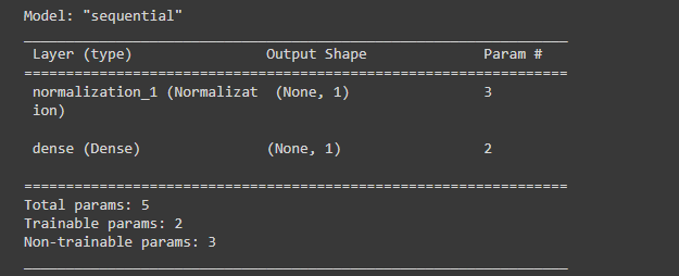这段代码定义了一个包含一个输入层、一个隐藏层和一个输出层的简单神经网络模型，用于预测汽车的燃油效率，具体来说：
（1）horsepower_normalizer 是一个 Keras 层，用于对训练集中的马力特征进行归一化处理。
（2）layers.Dense 是一个 Keras 层，用于定义全连接层，units=1 表示该层只有一个神经元，即模型的输出为一个标量值。
（3）tf.keras.Sequential 是一个 Keras 模型容器，用于按顺序堆叠各个层，构建模型。
（4）在 Sequential 容器中，首先添加了一个归一化层 horsepower_normalizer，用于对输入数据进行归一化处理；然后添加了一个全连接层 layers.Dense，用于从归一化后的马力特征中提取相关特征，并生成一个标量值作为模型的输出。
（5）summary 方法用于打印模型的摘要信息，包括模型的名称、输入形状、各层的名称、输出形状和参数个数等信息。
This model will predict ‘MPG’ from ‘Horsepower’.
Run the untrained model on the first 10 ‘Horsepower’ values. The output won’t be good, but notice that it has the expected shape of (10, 1):

horsepower_model.predict(horsepower[:10])

运行结果：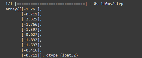

这段代码用于对训练集中的前10个样本的马力特征进行燃油效率预测，具体来说：
（1）horsepower 是一个包含训练集中马力特征的 NumPy 数组对象。
（2）horsepower[:10] 表示取出该数组中的前10个元素，即训练集中的前10个样本的马力特征。
（3）horsepower_model 是一个 Keras 模型，用于预测汽车的燃油效率。
（4）predict 方法用于对输入数据进行燃油效率预测，返回一个包含预测结果的 NumPy 数组对象。

Once the model is built, configure the training procedure using the Keras Model.compile method.
The most important arguments to compile are the loss and the optimizer, since these define what will be optimized (mean_absolute_error) and how (using the tf.keras.optimizers.Adam).

horsepower_model.compile(
    optimizer=tf.keras.optimizers.Adam(learning_rate=0.1),
    loss='mean_absolute_error')

这段代码用于编译神经网络模型，配置模型的优化器和损失函数，具体来说：
（1）horsepower_model 是一个 Keras 模型，用于预测汽车的燃油效率。
（2）compile 方法用于编译模型，其中可以指定优化器和损失函数等参数。
（3）optimizer 参数用于指定优化器，这里使用了 Adam 优化器，learning_rate=0.1 表示学习率为 0.1。
（4）loss 参数用于指定损失函数，这里使用了平均绝对误差（MAE）作为损失函数。

Use Keras Model.fit to execute the training for 100 epochs:

history = horsepower_model.fit(
    train_features['Horsepower'],
    train_labels,
    epochs=100,
    # Suppress logging.
    verbose=0,
    # Calculate validation results on 20% of the training data.
    validation_split = 0.2)

运行结果：

这段代码用于对神经网络模型进行训练，具体来说：
（1）horsepower_model 是一个 Keras 模型，用于预测汽车的燃油效率。
（2）fit 方法用于对模型进行训练，其中需要指定训练数据、标签、训练轮数和验证集等参数。
（3）train_features[‘Horsepower’] 表示训练集中的马力特征列，用于作为模型的输入数据进行训练。
（4）train_labels 是一个包含训练集中燃油效率标签的 NumPy 数组对象，用于作为模型的输出数据进行训练。
（5）epochs 参数用于指定训练轮数，这里为 100 轮。
（6）verbose 参数用于控制训练过程的详细程度，verbose=0 表示不输出训练日志信息。
（7）validation_split 参数用于指定验证集的比例，这里为 0.2，表示使用训练集的 20% 作为验证集。

Visualize the model’s training progress using the stats stored in the history object:

hist = pd.DataFrame(history.history)
hist['epoch'] = history.epoch
hist.tail()

运行结果：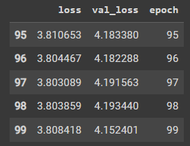

这段代码用于将训练历史记录保存为一个 Pandas DataFrame 对象，方便后续进行可视化和分析，具体来说：
（1）history 是一个包含训练历史记录的 Keras 对象，其中包括了训练过程中的损失函数值和验证集损失函数值的变化情况等信息。
（2）history.history 属性是一个字典对象，其中包含了训练过程中损失函数值和验证集损失函数值的变化情况，可以通过将该属性转换为 Pandas DataFrame 对象，来方便地进行后续的可视化和分析。
（3）pd.DataFrame 是 Pandas 库中的一个函数，用于将字典对象转换为 DataFrame 对象，从而方便进行数据处理和可视化。
（4）hist[‘epoch’] = history.epoch 表示将训练轮数作为一个新的列添加到 DataFrame 对象中，方便后续进行可视化和分析。
（5）hist.tail() 方法用于查看 DataFrame 对象的最后五行，以了解训练历史记录的最终状态，包括训练轮数、训练集损失函数值、验证集损失函数值等信息。
（6）因此，该代码的作用是将训练历史记录保存为一个 Pandas DataFrame 对象，并查看其中的最后五行，以了解训练过程中的损失函数值和验证集损失函数值等信息。这可以用于评估模型的训练效果和调整模型的超参数。

def plot_loss(history):
  plt.plot(history.history['loss'], label='loss')
  plt.plot(history.history['val_loss'], label='val_loss')
  plt.ylim([0, 10])
  plt.xlabel('Epoch')
  plt.ylabel('Error [MPG]')
  plt.legend()
  plt.grid(True)

这段代码定义了一个名为 plot_loss 的函数，用于绘制模型训练过程中的损失函数值和验证集损失函数值的变化情况，具体来说：
（1）history 是一个包含训练历史记录的 Keras 对象，其中包括了训练过程中的损失函数值和验证集损失函数值的变化情况等信息。
（2）plt.plot 方法用于绘制折线图，其中 history.history[‘loss’] 表示训练集损失函数值的变化情况，history.history[‘val_loss’] 表示验证集损失函数值的变化情况。
（3）plt.ylim 方法用于设置 y 轴坐标的取值范围，这里限定在 0 到 10 的范围内，方便比较不同模型的训练效果。
（4）plt.xlabel 和 plt.ylabel 方法用于设置 x 轴和 y 轴的标签。
（5）plt.legend 方法用于添加图例，其中 label 参数表示图例的文本标签。
（6）plt.grid 方法用于添加网格线，方便比较不同模型的训练效果。

plot_loss(history)

运行结果：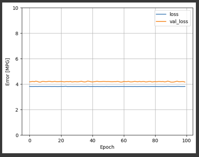

这段代码调用了刚才定义的 plot_loss 函数，用于绘制模型训练过程中的损失函数值和验证集损失函数值的变化情况，具体来说：
（1）plot_loss 是一个函数，用于绘制模型训练过程中的损失函数值和验证集损失函数值的变化情况。
（2）history 是一个包含训练历史记录的 Keras 对象，其中包括了训练过程中的损失函数值和验证集损失函数值的变化情况等信息。
（3）plot_loss(history) 表示调用 plot_loss 函数，并传入一个包含训练历史记录的 Keras 对象 history，以绘制相应的折线图。

Collect the results on the test set for later:

test_results = {}

test_results['horsepower_model'] = horsepower_model.evaluate(
    test_features['Horsepower'],
    test_labels, verbose=0)

这段代码用于测试已经训练好的模型在测试集上的表现，具体来说：
（1）test_results 是一个字典对象，用于保存不同模型在测试集上的表现，其中键为模型的名称，值为模型在测试集上的评估结果。
（2）horsepower_model 是一个 Keras 模型，用于预测汽车的燃油效率。
（3）evaluate 方法用于对模型在测试集上进行评估，其中需要指定测试数据和标签等参数。
（4）test_features[‘Horsepower’] 表示测试集中的马力特征列，用于作为模型的输入数据进行评估。
（5）test_labels 是一个包含测试集中燃油效率标签的 NumPy 数组对象，用于作为模型的输出数据进行评估。
（6）verbose 参数用于控制评估过程的详细程度，verbose=0 表示不输出评估日志信息。

Since this is a single variable regression, it’s easy to view the model’s predictions as a function of the input:

x = tf.linspace(0.0, 250, 251)
y = horsepower_model.predict(x)

运行结果：

这段代码用于使用已经训练好的模型对给定的输入数据进行预测，具体来说：
（1）tf.linspace 是 TensorFlow 库中的一个函数，用于生成一个均匀分布的一维张量。其中，0.0 表示起始值，250 表示终止值，251 表示生成的张量的长度。
（2）x 是一个包含从 0.0 到 250 之间的等间隔数值的一维张量，用于作为模型的输入数据进行预测。
（3）horsepower_model 是一个 Keras 模型，用于预测汽车的燃油效率。
（4）predict 方法用于对模型进行预测，其中需要指定输入数据。
（5）y 是一个包含模型对输入数据进行预测的结果的一维张量，用于表示模型预测的结果，具有与输入数据 x 相同的长度。

def plot_horsepower(x, y):
  plt.scatter(train_features['Horsepower'], train_labels, label='Data')
  plt.plot(x, y, color='k', label='Predictions')
  plt.xlabel('Horsepower')
  plt.ylabel('MPG')
  plt.legend()

这段代码用于绘制模型在训练集和测试集上的预测结果，并将其与原始数据进行比较，具体来说：
（1）plot_horsepower 是一个函数，用于绘制模型在训练集和测试集上的预测结果，并将其与原始数据进行比较。
（2）x 是一个包含从 0.0 到 250 之间的等间隔数值的一维张量，用于表示模型的预测输入数据。
（3）y 是一个包含模型对输入数据进行预测的结果的一维张量，用于表示模型的预测输出数据。
（4）plt.scatter 方法用于绘制散点图，其中 train_features[‘Horsepower’] 和 train_labels 分别表示训练集中的马力特征列和燃油效率标签列，用于作为原始数据的输入和输出数据进行绘制。
（5）plt.plot 方法用于绘制折线图，其中 x 和 y 分别表示模型的预测输入和输出数据，用于绘制模型的预测结果。
（6）color 参数用于设置折线图的颜色，‘k’ 表示黑色。
（7）plt.xlabel 和 plt.ylabel 方法用于设置 x 轴和 y 轴的标签。
（8）plt.legend 方法用于添加图例，其中 label 参数表示图例的文本标签。

plot_horsepower(x, y)

运行结果：

Linear regression with multiple inputs
You can use an almost identical setup to make predictions based on multiple inputs.
This model still does the same y=mx+b except that m is a matrix and x is a vector.
Create a two-step Keras Sequential model again with the first layer being normalizer (tf.keras.layers.Normalization(axis=-1)) you defined earlier and adapted to the whole dataset:

linear_model = tf.keras.Sequential([
    normalizer,
    layers.Dense(units=1)
])

这段代码定义了一个简单的线性回归模型，采用了 Keras 中的 Sequential 模型 API，具体来说：
（1）tf.keras.Sequential 是一个 Sequential 模型类，用于按顺序堆叠各种神经网络层，构建深度神经网络模型。
（2）normalizer 是一个用于标准化输入数据的层，用于将输入数据进行归一化处理，使其具有相似的分布和尺度，从而加速模型的训练和提高模型的精度。
（3）layers.Dense 是一个全连接层类，用于实现神经网络中的全连接操作。其中，units=1 表示该层的输出维度为 1，即该模型只有一个输出节点，因为这是一个回归模型，用于预测连续的数值型目标变量。
（4）linear_model 是一个 Sequential 模型对象，由 normalizer 层和 Dense 层按顺序堆叠而成，用于实现线性回归模型。

When you call Model.predict on a batch of inputs, it produces units=1 outputs for each example:

linear_model.predict(train_features[:10])

运行结果：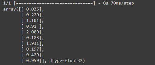

这段代码用于对已经训练好的线性回归模型 linear_model 对训练集中的前 10 个样本进行预测，具体来说：
（1）linear_model 是一个已经训练好的线性回归模型，用于预测汽车的燃油效率。
（2）predict 方法用于对模型进行预测，其中需要指定输入数据。
（3）train_features 是一个包含训练集中各个特征列的 NumPy 数组对象，用于作为模型的输入数据进行预测。
（4）train_features[:10] 表示训练集中前 10 个样本的特征数据，用于作为模型的输入数据进行预测。
（5）linear_model.predict(train_features[:10]) 表示对训练集中前 10 个样本的特征数据进行预测，并返回模型的预测结果，这里是一个包含 10 个元素的 NumPy 数组对象。

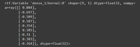
When you call the model, its weight matrices will be built—check that the kernel weights (the m in y=mx+b ) have a shape of (9, 1):

linear_model.layers[1].kernel

Configure the model with Keras Model.compile and train with Model.fit for 100 epochs:

linear_model.compile(
    optimizer=tf.keras.optimizers.Adam(learning_rate=0.1),
    loss='mean_absolute_error')

这段代码用于编译一个已经定义好的 Keras 模型 linear_model，指定优化器和损失函数，具体来说：
（1）compile 方法用于编译一个已经定义好的 Keras 模型，指定优化器和损失函数等模型训练的相关参数。
（2）optimizer 参数用于指定优化器，这里采用了 Adam 优化器，其学习率为 0.1。
（3）tf.keras.optimizers.Adam 是 Adam 优化器的实现类，用于训练神经网络模型，其学习率 learning_rate=0.1 表示每次参数更新的步长大小。
（4）loss 参数用于指定损失函数，这里采用了平均绝对误差（MAE）作为损失函数。
（5）‘mean_absolute_error’ 表示平均绝对误差（MAE）损失函数，用于评估模型的预测结果与真实值之间的差异。

history = linear_model.fit(
    train_features,
    train_labels,
    epochs=100,
    # Suppress logging.
    verbose=0,
    # Calculate validation results on 20% of the training data.
    validation_split = 0.2)

这段代码用于训练已经编译好的线性回归模型 linear_model，并返回训练历史信息，具体来说：
（1）linear_model 是一个已经编译好的线性回归模型，用于预测汽车的燃油效率。
（2）fit 方法用于训练模型，其中需要指定训练数据和训练参数等相关信息。
（3）train_features 是一个包含训练集中各个特征列的 NumPy 数组对象，用于作为模型的训练输入数据。
（4）train_labels 是一个包含训练集中标签列的 NumPy 数组对象，用于作为模型的训练输出数据。
（5）epochs 参数用于指定训练的轮数，即将训练数据集的所有样本都使用一次作为训练的一轮。
（6）verbose 参数用于指定训练过程中的输出信息等级，verbose=0 表示不输出任何训练信息。
（7）validation_split 参数用于指定验证集的比例，这里指定为 0.2，表示将训练集中的 20% 作为验证集，用于评估模型的性能和防止过拟合。
（8）history 是一个字典对象，包含了训练过程中的历史信息，如损失函数的值、指标的值等。

Using all the inputs in this regression model achieves a much lower training and validation error than the horsepower_model, which had one input:

plot_loss(history)

运行结果：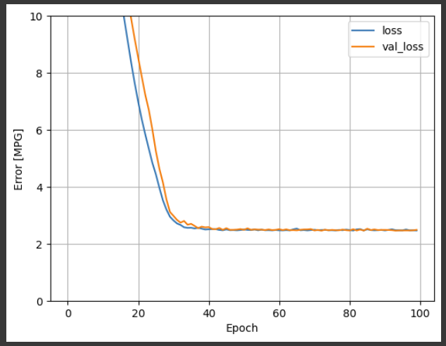

Collect the results on the test set for later:

test_results['linear_model'] = linear_model.evaluate(
    test_features, test_labels, verbose=0)

Regression with a deep neural network (DNN)
Here, you will implement single-input and multiple-input DNN models.
在这里，你将实现单输入和多输入的DNN模型。
The code is basically the same except the model is expanded to include some “hidden” non-linear layers.
除了模型被扩展到包括一些 "隐藏的 "非线性层之外，代码基本上是相同的。
The name “hidden” here just means not directly connected to the inputs or outputs.
这里的 "隐藏 "只是指不直接连接到输入或输出。
These models will contain a few more layers than the linear model:

（1）The normalization layer, as before (with horsepower_normalizer for a single-input model and normalizer for a multiple-input model).
（2）Two hidden, non-linear, Dense layers with the ReLU (relu) activation function nonlinearity.
（3）A linear Dense single-output layer.
归一化层，和以前一样（单输入模型用horpower_normalizer，多输入模型用normalizer）。
两个隐藏的、非线性的、具有ReLU（relu）激活函数非线性的Dense层。
一个线性的Dense单输出层。
Both models will use the same training procedure, so the compile method is included in the build_and_compile_model function below.
两个模型将使用相同的训练过程，所以编译方法包含在下面的build_and_compile_model函数中。

def build_and_compile_model(norm):
  model = keras.Sequential([
      norm,
      layers.Dense(64, activation='relu'),
      layers.Dense(64, activation='relu'),
      layers.Dense(1)
  ])

  model.compile(loss='mean_absolute_error',
                optimizer=tf.keras.optimizers.Adam(0.001))
  return model

这段代码定义了一个函数build_and_compile_model，该函数接受一个名为norm的参数，该参数是一个用于标准化输入数据的预处理层。
函数实现了一个包含三个全连接层的神经网络模型，其中每个层的输出都是具有64个单元的张量，并使用ReLU激活函数进行非线性变换。最后一个层的输出是一个单元，用于回归问题的预测。
该模型使用均方误差（MSE）作为损失函数，并使用Adam优化器进行模型参数的更新，学习率为0.001。最终返回编译好的模型以供训练和评估使用。
具体来说，以下是函数中每个组成部分的详细说明：
（1）keras.Sequential：该函数创建了一个顺序模型，它是多个神经网络层的线性堆叠，其中每个层都有一个输入张量和一个输出张量。
（2）norm：输入数据的标准化是通过norm参数传递的预处理层实现的，该层将在模型的第一层中使用。
（3）layers.Dense：这是一个密集连接层，它将输入张量与权重矩阵相乘，再加上偏置向量，然后应用激活函数。
（4）activation=‘relu’：ReLU激活函数是一种非线性变换，它将所有负值都变为零，保留所有正值不变。这有助于模型学习更加复杂的非线性关系。
（5）loss=‘mean_absolute_error’：这是模型的损失函数，用于衡量模型的预测值与真实值之间的差距。在这里，使用的是平均绝对误差（MAE）作为损失函数，它是预测值与真实值之间差的绝对值的平均值。
（6）optimizer=tf.keras.optimizers.Adam(0.001)：Adam是一种常用的优化算法，用于更新模型参数以最小化损失函数。在这里，使用Adam优化器，学习率为0.001。
（7）return model：将编译好的模型返回以供训练和评估使用。
Regression using a DNN and a single input
Create a DNN model with only ‘Horsepower’ as input and horsepower_normalizer (defined earlier) as the normalization layer:
创建一个只有 "Horsepower "作为输入的DNN模型，将horsepower_normalizer（前面定义的）作为归一化层：

dnn_horsepower_model = build_and_compile_model(horsepower_normalizer)

这段代码创建了一个名为dnn_horsepower_model的深度神经网络模型，并使用build_and_compile_model函数对其进行编译。其中，horsepower_normalizer是用于标准化输入数据的预处理层。
（1）build_and_compile_model(horsepower_normalizer)：调用build_and_compile_model函数创建一个深度神经网络模型，并传递horsepower_normalizer作为预处理层。horsepower_normalizer是一个用于标准化输入特征的tf.keras.layers.experimental.preprocessing.Normalization层，用于将输入特征缩放到均值为0，标准差为1的标准正态分布。
（2）dnn_horsepower_model = …：将编译好的深度神经网络模型赋值给名为dnn_horsepower_model的变量，以便在后续的训练和预测中使用该模型。
This model has quite a few more trainable parameters than the linear models:
这个模型比线性模型多了不少可训练的参数：

dnn_horsepower_model.summary()

运行结果：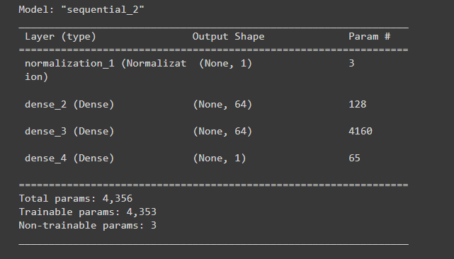

.summary()：这是一个tf.keras.models.Model类的方法，用于打印模型的概述信息。该方法将输出模型的层次结构、每层的输出形状、参数数量和可训练性等信息。

打印出的模型概述信息通常包括以下内容：

Model: 模型的名称和类型。
Layer (type): 每个层的名称和类型。
Output Shape: 每个层的输出形状。
Param #：每个层的参数数量。
Trainable: 每个层是否可训练。
Train the model with Keras Model.fit:
用Keras Model.fit训练模型：

history = dnn_horsepower_model.fit(
    train_features['Horsepower'],
    train_labels,
    validation_split=0.2,
    verbose=0, epochs=100)

运行结果：

（1）dnn_horsepower_model.fit()：这是深度神经网络模型的训练方法，用于训练模型并返回训练历史记录。
（2）train_features[‘Horsepower’]：这是训练集中的一个特征列，用于训练模型。在这里，我们使用Horsepower特征列来训练模型。
（3）train_labels：这是训练集中的标签列，用于训练模型。在这里，我们使用train_labels列来训练模型，这是每个样本的真实值。
（4）validation_split=0.2：这是将训练集划分为训练和验证集的一种方法，其中validation_split参数指定了要用作验证集的数据集的比例。在这里，我们将20%的训练数据用作验证集，其余80%用于模型的训练。
（5）verbose=0：这个参数用于控制模型训练时输出的详细程度。在这里，我们将其设置为0，表示不输出任何信息。
（6）epochs=100：这个参数指定了训练过程中要运行的迭代次数。在这里，我们将模型训练100个epoch（即100次迭代）。
（7）history = dnn_horsepower_model.fit(…)：将训练历史记录存储在history变量中，以供后续的分析和可视化使用。
This model does slightly better than the linear single-input horsepower_model:
这个模型比线性单输入的马力_模型做得略好：

plot_loss(history)

If you plot the predictions as a function of ‘Horsepower’, you should notice how this model takes advantage of the nonlinearity provided by the hidden layers:
如果你把预测值绘制成 "马力 "的函数，你应该注意到这个模型是如何利用隐藏层提供的非线性的：

x = tf.linspace(0.0, 250, 251)
y = dnn_horsepower_model.predict(x)

运行结果：

plot_horsepower(x, y)

运行结果：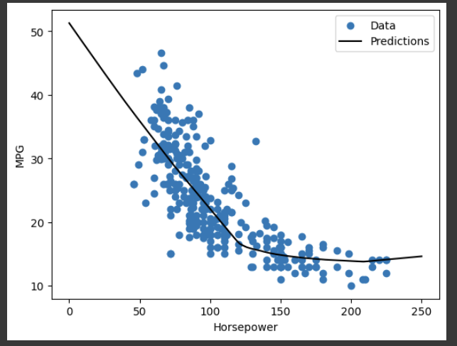

Collect the results on the test set for later:

test_results['dnn_horsepower_model'] = dnn_horsepower_model.evaluate(
    test_features['Horsepower'], test_labels,
    verbose=0)

Regression using a DNN and multiple inputs
Repeat the previous process using all the inputs. The model’s performance slightly improves on the validation dataset.

dnn_model = build_and_compile_model(normalizer)
dnn_model.summary()

运行结果：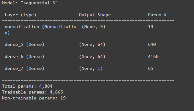

history = dnn_model.fit(
    train_features,
    train_labels,
    validation_split=0.2,
    verbose=0, epochs=100)

运行结果：

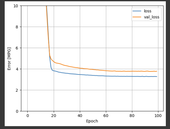
plot_loss(history)

运行结果：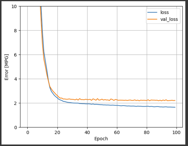

Collect the results on the test set:

test_results['dnn_model'] = dnn_model.evaluate(test_features, test_labels, verbose=0)

Performance
Since all models have been trained, you can review their test set performance:
由于所有模型都已被训练，你可以审查它们的测试集性能：

pd.DataFrame(test_results, index=['Mean absolute error [MPG]']).T

运行结果：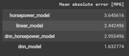

These results match the validation error observed during training.
Make predictions
You can now make predictions with the dnn_model on the test set using Keras Model.predict and review the loss:
现在你可以用Keras Model.predict对测试集的dnn_model进行预测，并查看损失：

test_predictions = dnn_model.predict(test_features).flatten()

a = plt.axes(aspect='equal')
plt.scatter(test_labels, test_predictions)
plt.xlabel('True Values [MPG]')
plt.ylabel('Predictions [MPG]')
lims = [0, 50]
plt.xlim(lims)
plt.ylim(lims)
_ = plt.plot(lims, lims)

运行结果：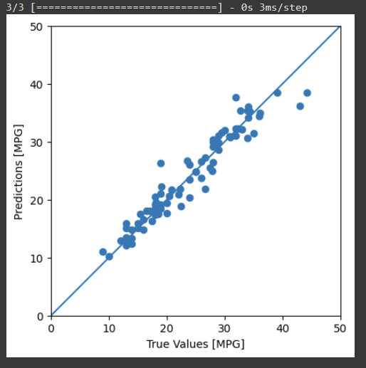

It appears that the model predicts reasonably well.

Now, check the error distribution:

error = test_predictions - test_labels
plt.hist(error, bins=25)
plt.xlabel('Prediction Error [MPG]')
_ = plt.ylabel('Count')

运行结果：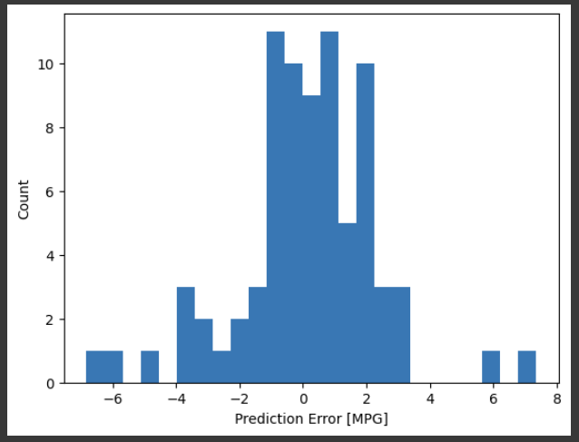

If you’re happy with the model, save it for later use with Model.save:

dnn_model.save('dnn_model.keras')